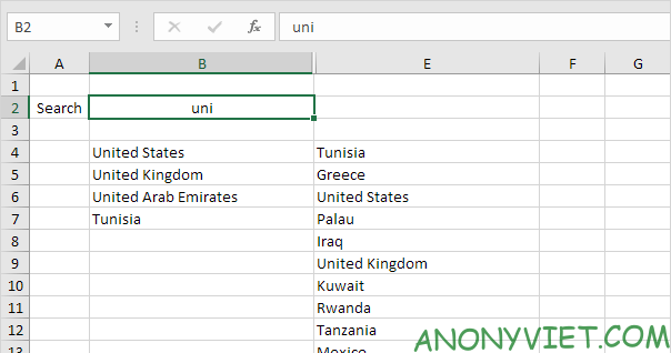
In this article, I will show you how to create your own search dialog in Excel. If you enter a search command in cell B2, Excel will search through column E and the results appear in column B.
| Join the channel Telegram of the AnonyViet 👉 Link 👈 |

How to Create a Search Dialog in Excel
first. Select cell D4 and type the command SEARCH absolute reference to cell B2.
2. Double-click the lower-right corner of cell D4 to quickly copy the function to other cells.
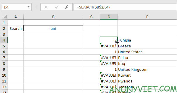
Explanation: the SEARCH function is used to find the position of a substring in a string. The SEARCH function is not case sensitive. For Tunisia, the string “uni” is found at position 2. For the United States, the string “uni” is found at position 1. The lower the position, the higher the ranking.
3. Both United States and United Kingdom return 1 (duplicate). Adjust the formula as shown below to remove error cells.
4. Again, double-click the lower-right corner of cell D4 to quickly copy the formula to other cells.
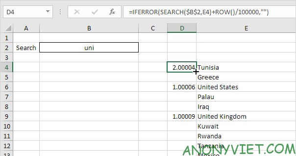
Explain: jaw ROW Returns the row number of the cell. If we divide the number of rows by a large number and add it to the result of the function SEARCHwe will have non-duplicate values of cells in the same position.
However, these small numbers will not affect search rankings. United States currently has a value of 1,00006 and United Kingdom has a value of 1,00009. We also added the IFERROR function. If a cell has an error (when the string is not found), it is left blank (“”).
5. Select cell C4 and insert the RANK function as shown below.
6. Double-click the lower-right corner of cell C4 to quickly copy the formula to other cells.
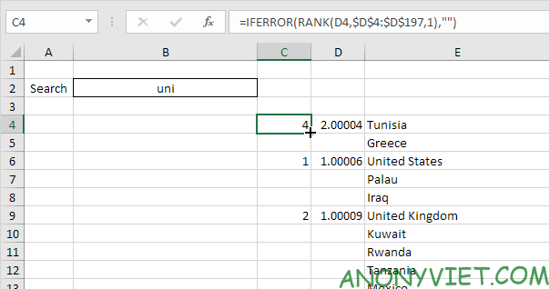
Explain: The RANK function returns the rank of a number. If the third argument is 1, Excel will rank in ascending, . Since we added the ROW function, all values in column D are unique. Therefore, the ranks in column C are also unique (no constraints).
7. We will use the VLOOKUP function to return the countries found (lowest ranking first,…) Select cell B4 and insert the VLOOKUP function shown below.
8. Double-click the lower-right corner of cell B4 to quickly copy the formula to other cells.
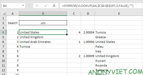
9. Change the text color of the numbers in column A to white and hide columns C and D.
Result:
In addition, you can also view many other excel articles here.


