This article will show you how to use the GetPivotData function in Excel.
| Join the channel Telegram of the AnonyViet 👉 Link 👈 |
In this article, I will show you how to use the GetPivotData function.
You can download the test file here: link
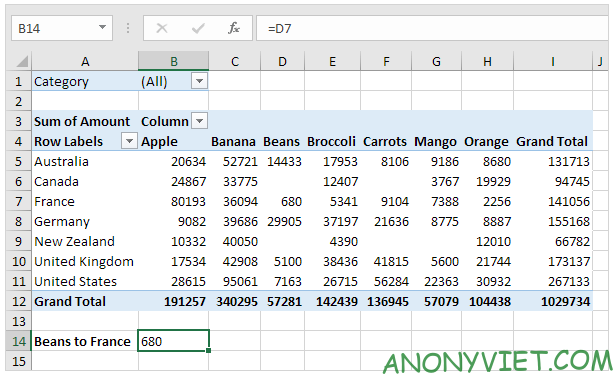
1. First, select cell B14 below and enter =D7 (don’t click on cell D7 in the Pivot table) to reference the number of beans exported to France.
2. Use filter to show only the amount of vegetables exported to countries.
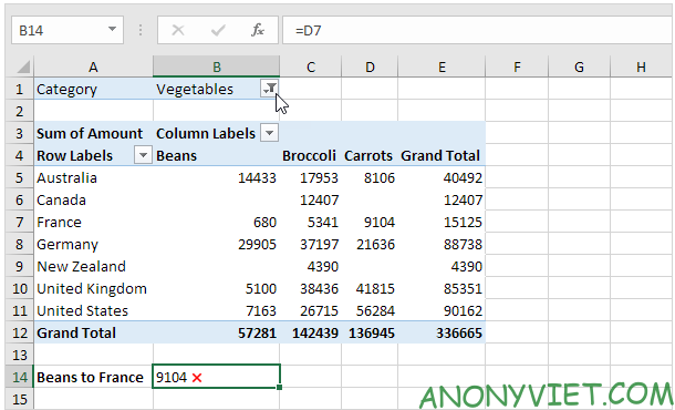
Note: cell B14 is currently referring to the amount of carrots exported to France, not the amount of beans.
3. Remove Filter. Select cell B14 again, type the equal sign (=) and click cell D7 in the Pivot table.
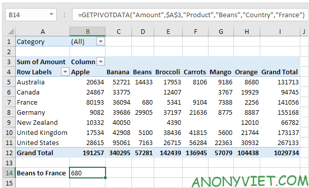
Note: Excel will automatically insert the GETPIVOTDATA function shown above.
4. And do it again use Filter to display the number of vegetables exported to each country.
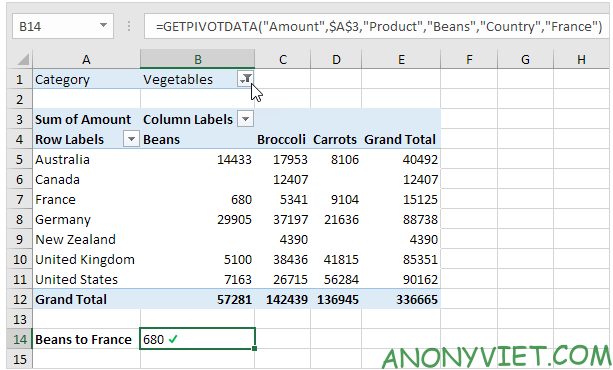
Note: the GETPIVOTDATA function returns the exact amount of beans exported to France.
5. The GETPIVOTDATA function can only return display data. For example, use Filter to show only the amount of fruit exported to each country.
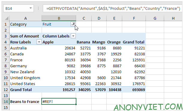
Note: the GETPIVOTDATA function returns the #REF! error because the value 680 is not displayed.
6. The dynamic GETPIVOTDATA function below returns the number of mangoes exported to Canada.
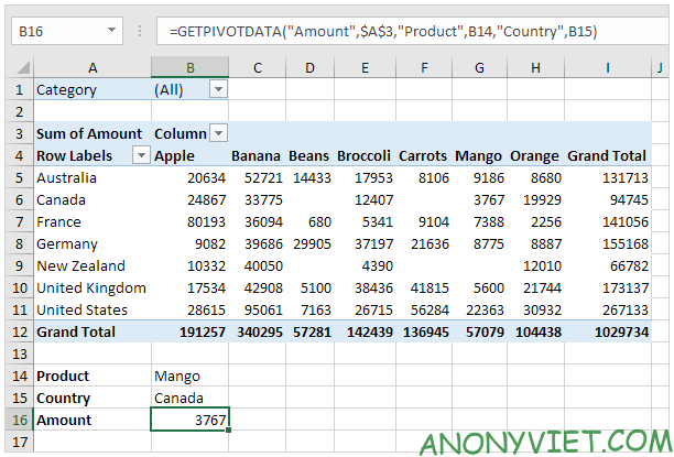
7. The GETPIVOTDATA function below has 4 values and returns the total amount exported to the US.
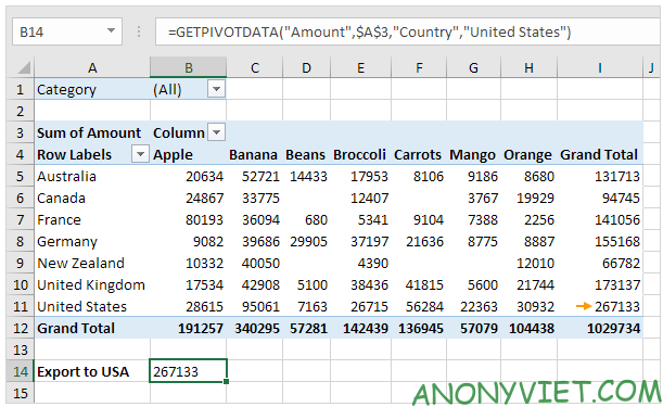
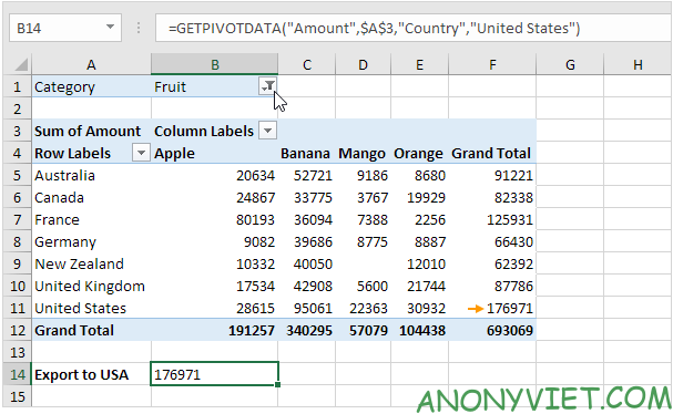
8. If the total amount exported to the United States changes (for example, by using filter), the value returned by the GETPIVOTDATA function also changes.
9. Click a cell in the Pivot Table
10. On the Analyze tab, click the drop-down arrow next to Options and uncheck Generate GetPivotData.


