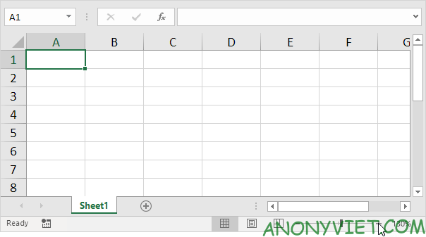
Status bar (status bar) in Excel can be quite useful. By default, the status bar at the bottom of the window shows the average, count, and sum of the selected cells.
| Join the channel Telegram of the AnonyViet 👉 Link 👈 |

How to use the Status Bar in Excel
Select from cell A1 to cell A3.

At the bottom of the screen, you’ll see a status bar next to average, count, and sum.

To change the view of the workbook, use the 3 shortcuts below on the status bar.

Use the zoom bar on the status bar to quickly zoom in or out to a desired ratio.
Customize Status Bar
Many status bar options are selected by default. You can right-click on the status bar to activate even more options.
First, right-click the status bar.
In this example, I will choose Caps Lock.

Note: This does not enable Caps Lock (see image above, Caps Lock is still off). Excel displays the Caps Lock status in the status bar.
Now press the Caps Lock key from the keyboard.
Excel will display Caps Lock in the status bar.

Right-click the status bar. Next, I will choose Minimum.
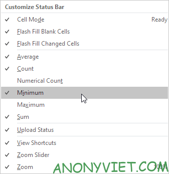
Select the area A1:A3.

You will now see the lowest value of the area you selected (Min).

Interesting Secrets of Status Bar
Here’s a little status bar secret: Excel uses the status bar in a variety of situations. If you don’t like that, you can hide the status bar.
In this example, we will filter the table.
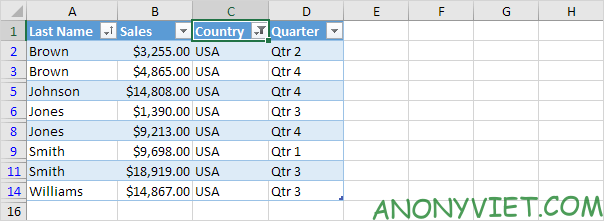
Excel uses the status bar to display the number of cells visible in the table.

Hover over a cell with one or more comments.
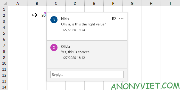
Excel uses the status bar to display the author’s name.

If you use Excel 2016, press the keyboard shortcut CTRL + SHIFT + F1 to hide the ribbon and status bar.
To hide only the status bar, add the following line of code in Workbook Open Events:
Application.DisplayStatusBar = False
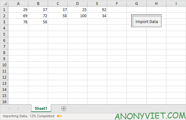
Use the StatusBar property in Excel VBA to display a status bar message.
In addition, you can also view many other excel articles here.


