There are three shortcuts in the top menu, which are Save, Undo and Back. However, if you want to use more keyboard shortcuts, like Copy and Cut, you can set them up like this:
File->Options->Quick Access Toolbar, add Cut and Copy from the left column to the right. You will see two more shortcuts added in the top menu.

5. Add a diagonal line to a cell
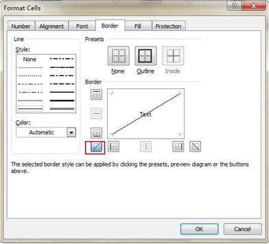
Diagonals in cells can separate different contents of rows and columns. You guys come in Home-> Font-> Borders and click More Borders.
6. Add more than one new row or column
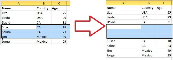
If you want to insert multiple rows or columns, just highlight x rows/columns and then right-click and click Insert. If you want to insert 3 rows then highlight 3 rows.
7. Quickly move and copy data in cells
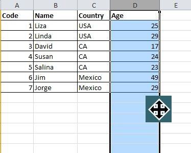
If you want to move a column of data, the quick way is to select that column and move the cursor to the border, after the cursor changes to the cross arrow icon, you can move the column freely. If you want to copy then press Ctrl button before dragging to move, the new column will copy all selected data.
8. Quickly delete empty cells
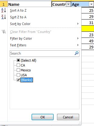
If you need to delete empty cells then a quick way is to filter out all blank cells and delete them with the mouse. Select the column you want to filter, go to Data->Filter, and select the last option, Blanks. All empty cells will be displayed immediately. Now you just need to delete them.
9. Wildcard search with Wild Card
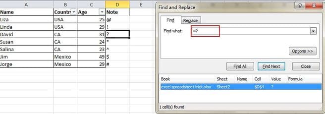
Wild Card search is a relative search, not 100% accurate results. For example, Wild Card has 3 main characters *, ? ~. They will replace characters we don’t know. Learn more about Wild Cards here.
10. Filter data by condition in column
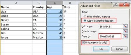
Advanced Filter is widely applied when you need to filter data according to certain conditions in a . Click to select the column and go to Data->Advanced. Click Copy to another locationcoordinates, you fill in the box Copy to. Don’t forget to select Unique records only, then click OK. You can also write filter conditions in cell Criteria range.
11. Check input data before input
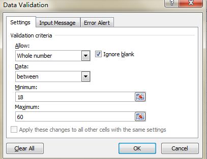
For example, age must be an integer, and all survey participants must be between 18 and 60 years old. To ensure that data that does not meet the above conditions is not accepted, you must restrict input, go to Data->Data Validation->Setting, enter the condition and switch to Input Message to give a prompt like “Please enter your age as an integer, this number will be in the range 18 to 60”. Users will receive this prompt when entering age is not eligible.
12. Navigate quickly with Ctrl + Arrow Keys
When you click Ctrl + any arrow button on the keyboard, you can jump to the last cell of the data. If you want to jump to the bottom line of the data, just click Ctrl + down arrow.

13. Move data from rows to columns
Transpose is a feature that will help you convert data from rows to columns quickly. Copy the area you want, move the cursor to another empty location. Go Home->Paste->Transposenote this function will not activate until you Copy (select data press Ctrl +) previous data.

14. Hide cell data
Almost all users know how to hide data by right clicking and selecting Hide, but this way is very easy to detect. The best and easiest way to hide data is to use the Format Cells function. Select the cell you want to hide and go to Open Format Cells->Number Tab>Custom->Enter ;;;-> Click OK, then all the values in the cell will be hidden and can only be seen in the toolbar awake.
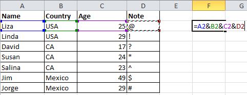
15. Merge text with &
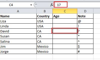
Sign & will help you to merge data in different cells into a new cell. As in the new box the result will be LizaUSA25@.
16. Convert font format
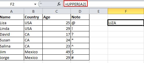
In excel, there are text formatting functions such as UPPER, LOWER and PROPER. UPPER will convert all letters to uppercase. LOWER will convert all text to lowercase. And PROPER will capitalize the first letter of each word.
17. Enter zero in the data box
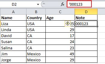
When you enter data with the first zero, Excel removes the zero by default. Instead of resetting the cell format, this problem can be easily solved by adding an apostrophe (‘) before the zero.
18. Shortcut feature with AutoCorrect
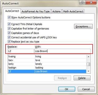
If you need to enter data more than once, you can use the feature AutoCorrect to turn acronyms into correct data. Take for example Liza Brown, which can be replaced by LZ. Therefore, every time I enter LZ, Excel will automatically correct it to Liza Brown. Into the File->Options->Proofing->AutoCorrect Options and enter the abbreviation in Replace and the exact data in With.
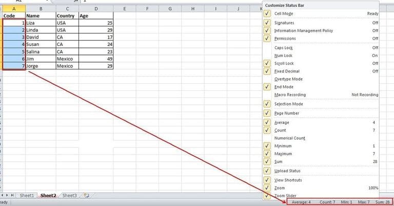
19. View Status
Most users know how to check the data status at the bottom of an Excel worksheet, such as Average and Average. However, did you know you can move the cursor to the bottom tab and right click to see more statuses?
20. Rename sheet by double click
There are many ways to rename a sheet and most users will right click to select Rename, which is very time consuming. The best way is just double click, then you can change the name directly.

In addition to these 20 tips that can turn you into an Excel expert, you can read more must-know Excel tips here.


