How to rename Columns or Rows in Google Sheets

If you’re creating a Google Sheets spreadsheet for someone else to use, and you want that person to easily find sections of data, you can use named ranges to change the column or row names. In this article, I will guide you to do so.

What are Named Ranges?

Named ranges allow you to rename columns or rows of a group of cells, an entire column or row. Renaming columns or rows does not overwrite the original cell references (A1, A2, etc.), but it does make it easier to refer to these cells (and the data within them) when you add new formulas.

Use Name Box

The fastest way to rename columns or rows in Google Sheet is to use Name Box. This is the cell to the left of the formula bar that shows you the cell reference or cells that are currently selected in your spreadsheet.

First, let’s open Google Sheets and select a new column or row. Then, replace the existing cell reference in the Name box with a new name, then press the Enter key to save the column or row name.

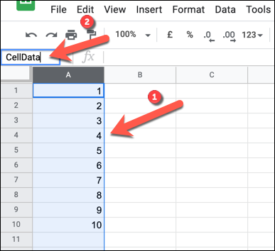
Google Sheet will apply the new name to your column or row immediately. You can view the list of available name ranges by clicking the down arrow button located to the right of the name box.

A list of named cells, including their original cell references, appears in the list below.

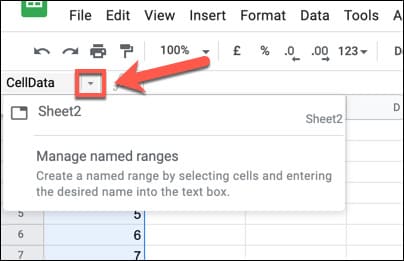
You can click on any name ranges to select those cells or press “Manage Named Ranges” to make changes to existing name ranges.

Another way to rename columns or rows is to use the Name Range menu. This menu allows you to manage existing name ranges as well as create new name ranges.

Add new name range

First, open Google Sheet and select the row or column you want to rename. Then, right-click on the selected cells and select “Define The Named Range”.

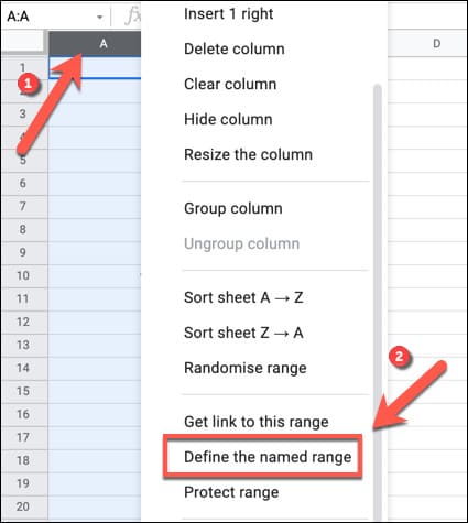
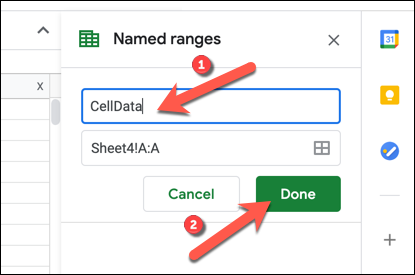
The “Named Ranges” menu will appear as a panel on the right. Enter your chosen name in the first box. You can also change the selected column, row, or cell range by changing the cell reference below.

Edit or delete Name Range

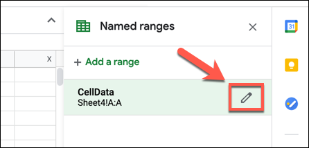
To edit or delete a name range, right-click any cell in the spreadsheet and select “Define Named Range”. You will see a list of available name ranges in the right panel. Hover over the name range you want and press the “Edit” button.

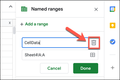
You can then make changes to the name range (including changing the name and cell range). If you want to remove the named range, press the “Remove” button.

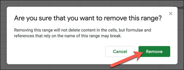
You need to confirm your choice — press “Remove” in the dialog box to confirm.

Use Name Range in Google Sheet

With the new name range added, you can now refer to this name range elsewhere in a new formula. For example, if you name your cell range “CellData,” you can find the average of the values ​​in those cells using the following formula:

=MEDIAN(CellData)

Name range (CellData) replaces cell references with columns, rows, or cell ranges in your formula. For example, if CellData is a name range of all the cells in column A, you can use A:A or CellData to refer to those cells.

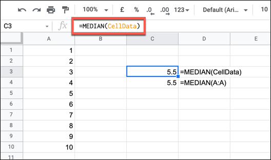
Using name range allows you to quickly refer to the data you want to use without requiring reference to the original cells. Also, if you don’t use Google Sheets, you can learn 20 Excel tricks that will turn you into an expert here.

Frequently asked questions

How can I rename columns or rows in Google Sheets?

You can rename columns or rows using the Name Box (the cell to the left of the formula bar) or the Name Range menu (by selecting the cell to be renamed, right-clicking and selecting “Define named range”).

What are Named Ranges and why should I use them?

Named Ranges allows you to name a group of cells, columns, or rows. This makes it easy to reference data in formulas, making your spreadsheet easier to read and understand.

How do I edit or delete a Named Range?

To edit or delete a Named Range, right-click any cell in the spreadsheet, select “Define named range”, find the Named Range to edit/delete and use the “Edit” or “Remove” button.