This article will show you how to use linear regression in Excel.
| Join the channel Telegram of the AnonyViet 👉 Link 👈 |
Linear regression
This literate teaches you how to use linear regression analysis in Excel and how to interpret the Summary Output.
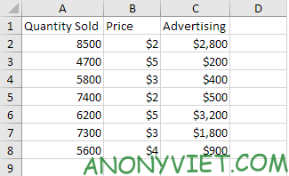
You can see the data below. The big question is: is there a relationship between Quantity Sold (Output) and Price and Advertising (Input). In other words: can we predict Quantity Sold if we know Price and Advertising?

1. On the Data tab, select Data Analysis.

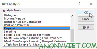
2. Select Regression and click OK.

3. Select Y Range (A1:A8). This is the predictor variable (also called the dependent variable).
4. Select X Range(B1:C8). These are the explanatory variables (also called independent variables). These columns must be adjacent to each other.
5. Check Labels.
6. Click Output Range and select cell A11.
7. Tick the Residuals box.
8. Press OK

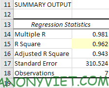
Excel generates the Summary Output as follows (rounded to 3 decimal places).
R Square
R Square is equal to 0.962, i.e. it fits very well. 96% of the variation in Quantity Sold is explained by the independent variables Price and Advertising. The closer to 1 the better the fit to the data.

The F and P values are significant
To check if your results are reliable (statistically significant), look at Significance F (0.001). If this value is less than 0.05, you are fine. If Significance F is greater than 0.05, it is probably better to stop using these independent variables. Delete a variable with a high P value (greater than 0.05) and run the regression again until the Significance F falls below 0.05.

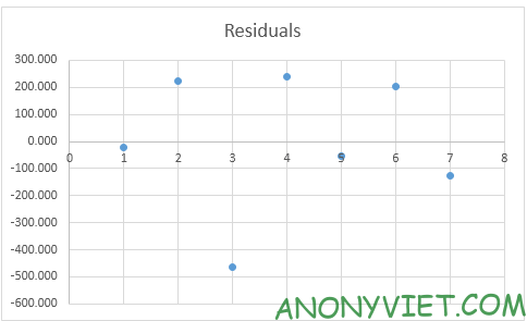
Residual
You can also create a scatter plot of these remainders.

In addition, you can also view many other excel articles here.


