Inserting a checkbox in Excel is very easy. For example, use checkboxes to create a dynamic checklist or chart. You can also insert a check mark symbol.
| Join the channel Telegram of the AnonyViet 👉 Link 👈 |

How to use Checkbox in Excel
First, open the Developer tab, in the Control section, select Insert.

Click Check Box in the Form Controls section.
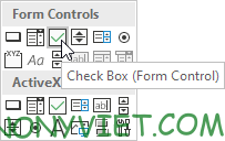
I will insert a checkbox in cell B2.

To remove “Check Box 1”, right-click the checkbox and click the text.

Checkbox link
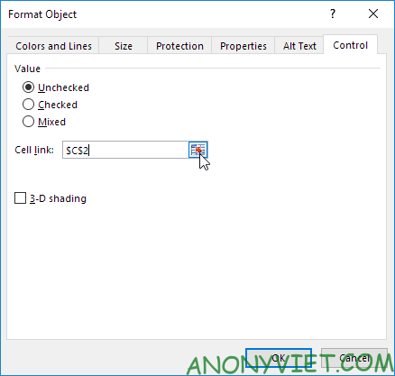
To associate a checkbox with a cell, perform the following steps.
Right-click the checkbox and select Format Control.
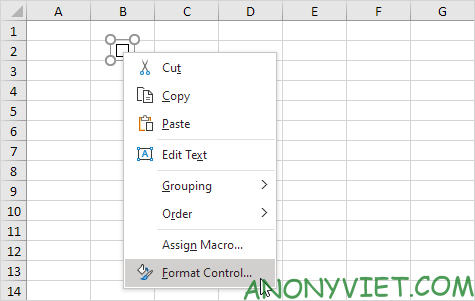
Link the checkbox to cell C2.
Check checkbox.
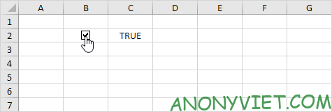
Next, I will hide column C.
And in this example, I will use the IF function.
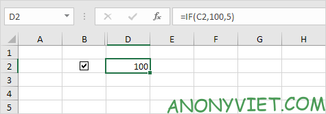
Uncheck the checkbox.
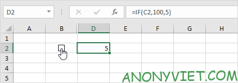
Explain a bit that cell C2 I have hidden, so you will not see, when selecting the checkbox, cell C2 will have the value True, so the if function in cell D2 will have the result 100. Conversely, when unchecking the checkbox, the cell C2 will have a value of False so cell D2 will have a result of 5.
How to create a Checklist
To create a checklist, you need to follow these steps.
First, insert a checkbox in cell B2.
Click the small square in the lower right corner in cell B2 and drag it down to cell B11.
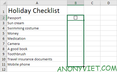
Right-click the checkbox and select Format Control.
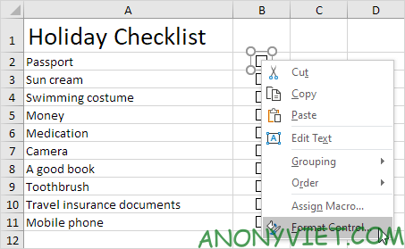
Link the checkbox to the cell next to it (cell C2).
Repeat the above action for all checkboxes.
Use the COUNTIF function to count selected checkboxes.
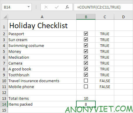
Hide column C. Then insert the IF function to check if all checkboxes are checked.
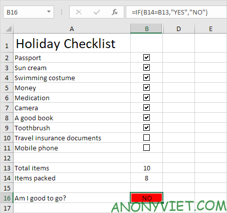
Select all checkboxes.
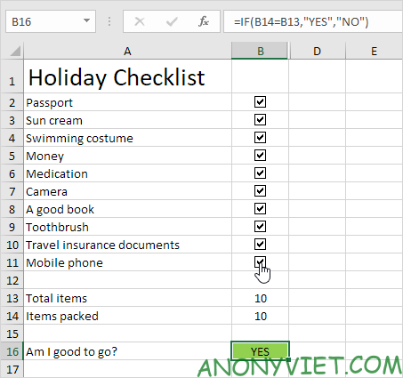
Note: I have use conditional formatting to automatically change cell background color B16.
Dynamic chart
Now I will apply checkboxes and dynamic charts to show you the practicality of checkboxes.
First, create a combo chart with two data series rainy day and profit (Rainy Days and Profit).
Next, insert 2 checkboxes.
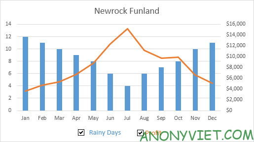
Right-click the first checkbox and select Format Control. Link this checkbox to cell B15.
Right-click the second checkbox and select Format Control. Link this checkbox to cell C15.
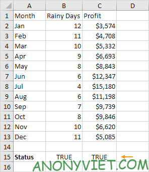
Uncheck the second checkbox. Cell C15 below changes to FALSE.
Now we will create two new data series by inserting the IF function below and copying this formula down to cell F13.
Repeat this step for the new Profit data.

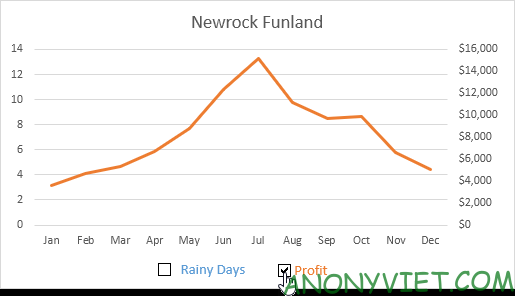
Explanation: if the checkbox is checked, the old and new data series are the same. If the checkbox is not selected, the new data series will change to the range with the #N/A error.
Use the new data series to create a combo chart. To do so, select the chart, right-click and select Select Data.
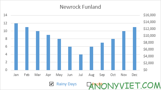
Uncheck the first checkbox and select the second checkbox.
How to clear checkbox
To delete multiple checkboxes at once, you just need to follow these steps.
Hold down Control and select the checkboxes you want to delete.
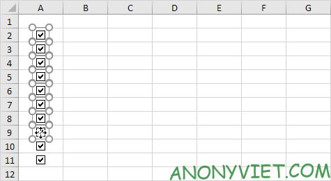
Then press Delete.
The power of checkboxes
Finally, you can also use VBA to create powerful checkboxes in Excel. Instead of inserting a Form control, insert an ActiveX control.
First, insert checkbox (ActiveX control).
Next, add the following two code snippets to hide and show column F.
If CheckBox1.Value = True Then Columns("F").Hidden = True
If CheckBox1.Value = False Then Columns("F").Hidden = False


In addition, you can also view many other excel articles here.


