This article will guide you to use Slicers to filter data in Excel.
| Join the channel Telegram of the AnonyViet 👉 Link 👈 |
This bouncing lesson will guide you to use Slicer to filter data.
1. Click a cell in a Pivot table
2. On the Analyze tab select Insert Slicer.

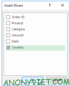
3. Select Country and Press OK
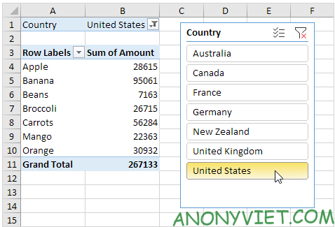
4. Click United States to find out which items are exported the most in the US
.
Next is the 2nd slice
5. Click a cell in the Pivot Table
6. On the Analyze tab select Insert Slicer.

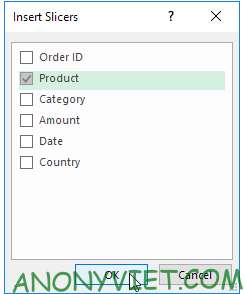
7. Select Product and Click OK
8 . select slicer
9. On the Options panel select a slicer style.

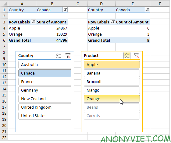
10. Use the second slicer. Click on Multi-Select and select multiple Products
11. Add a second Pivot Table.
12. Select the first slicer
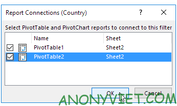
13. On the Options tab find and select Report Connections.

14. Select the second pivot table and click OK
15. Repeat steps 12-14 for the second slicer.
16. Use Both Slicers
In addition, you can also view many other excel articles here.


