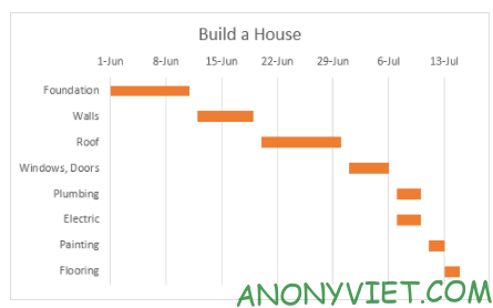
This article will show you how to create a Gantt chart in Excel.
| Join the channel Telegram of the AnonyViet 👉 Link 👈 |
Gantt charts
1. Select cell range A3:C11
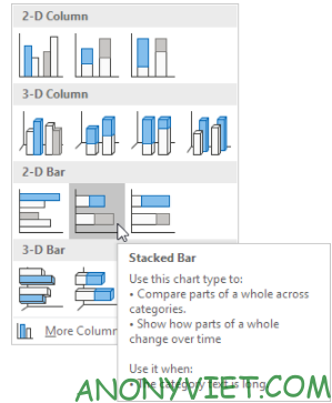
2. On the Insert tab, click the Columns icon.

3. Select Stacked Bar.
Result
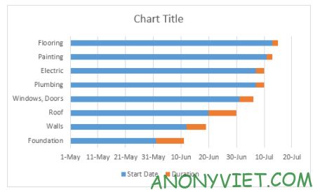
4. Enter a title by clicking the Chart Title. For example, Build a house.
5. Click the legend at the bottom and press Delete.
6. The tasks (Foundation, Walls, etc.) in reverse order. Right click on the tasks on the chart, click Format Axis and select ‘Categories in reverse order’.
Result
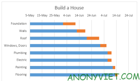
7. Right click on the blue bar, click Format Data Series, Fill & Line icon, Fill, No fill.
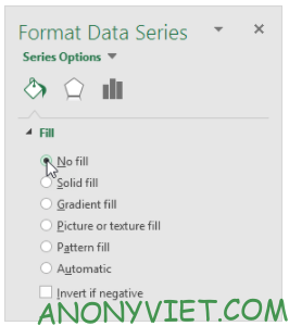
8. Date and time are stored as numbers in Excel and count the number of days since 0 Jan 1900. 1-jun-2017 (start) is like 42887. 15-jul-2017 (end) is like 42931. Right-click click on the date on the chart, click on Format Axis and change the minimum bound to 42887, maximum bound to 42931 and the Major unit to 7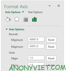
Result.
In addition, you can also view many other excel articles here.


