This article will show you how to create a pie chart in Excel.
| Join the channel Telegram of the AnonyViet 👉 Link 👈 |
Pie chart
This article will guide you to create a pie chart in Excel
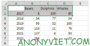
1. Select the range A1:D2.
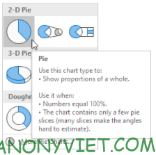
2. On the Insert tab, click the Circle icon.

3. Click on Pie
Result

Now will customize the chart to make it more beautiful.
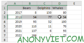
4. Select the range A1:D1, hold down the CTRL key, and select the range A3:D3.
5. Create a pie chart (steps 2 – 3)
6. Click the legend at the bottom and press Delete.
7. Select the pie chart.
8. Click the + sign to the right of the chart and click the box next to Data Label.

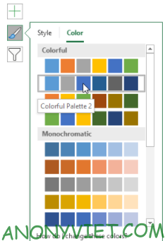
9. Click the brush icon on the right side of the chart and change the color of the chart.
Result

10. Right click on the pie chart and click Format Data Label.
11. Select Category Name, uncheck Value, select Percentage and press Center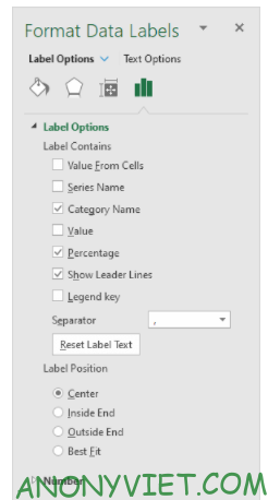
Result

In addition, you can also view many other excel articles here.


