In this article, I will show you how to use the SUMIF function in Excel.
| Join the channel Telegram of the AnonyViet 👉 Link 👈 |
How to use the SUMIF function in Excel
1. First we’ll start with a simple one. Example: I want to calculate the criteria of Facebook and Google in the table
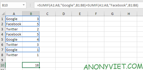
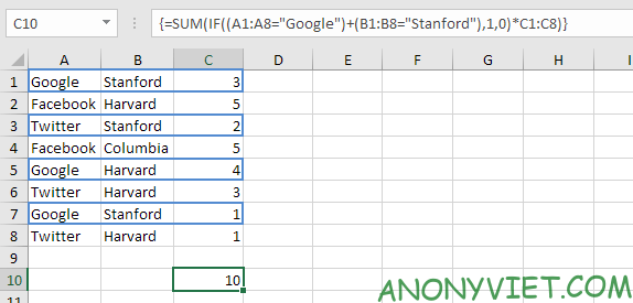
2 a. However, if we want to sum cells that meet the following criteria: Google or Stanford, we cannot use the SUMIF function twice (see figure below). Cells that meet Google and Stanford’s criteria are added twice, but they should only be added once.

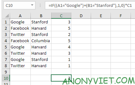
2b. We need an array of formulas. Here I will, use the IF function to check if Google or Stanford has an error
2 C. All you need is a SUM function to sum these values. To do this I will add the SUM function and replace A1 with A1:A8, B1 with B1:B8 and C1 with C1:C8.
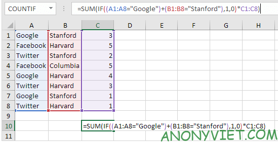
2d. Finish by pressing CTRL + SHIFT + ENTER.
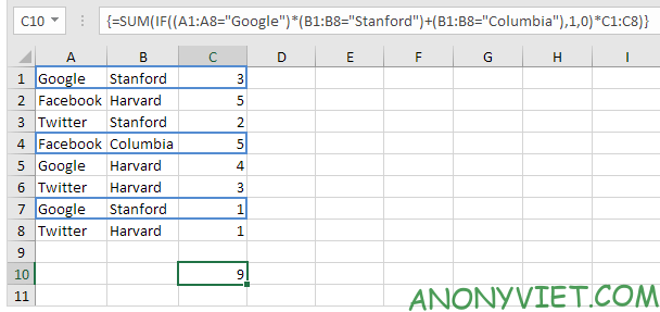
3. And I will do one more step. Here I will spread the following criteria: (Google and Stanford) or Columbia.
In addition, you can also view many other excel articles here.


