To look up a value in a two-way range, use INDEX and MATCH in Excel.
| Join the channel Telegram of the AnonyViet 👉 Link 👈 |
Two-way lookup in Excel
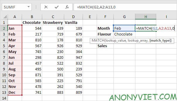
1. To find the position of February in the range A2:A13, use the MATCH function. The result is 2.
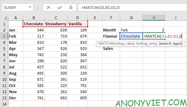
2. To find Chocolate’s position in the range B1:D1, use the MATCH function. The result is 1.
3. Use these results and the INDEX function to find February Chocolate sales.
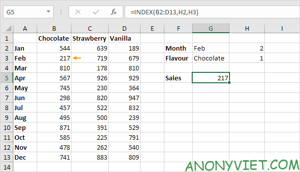
Explanation: 217 is found at the intersection of row 2 and column 1 in the range B2:D13.
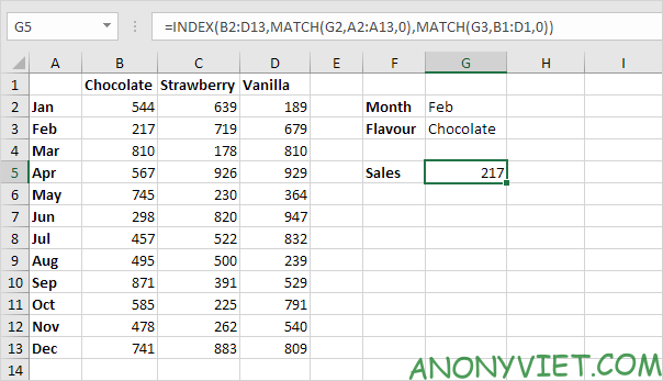
4. Combine it all together.
You can also look up a value in a two-way range without using INDEX and MATCH.
5. Select the range A1:D13.
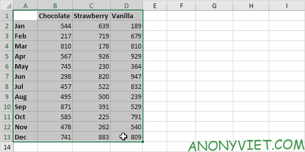
6. On the Formulas tab, in the Defined Names group, click Create from Selection.

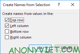
7. Select Top row and Left column and then click OK.
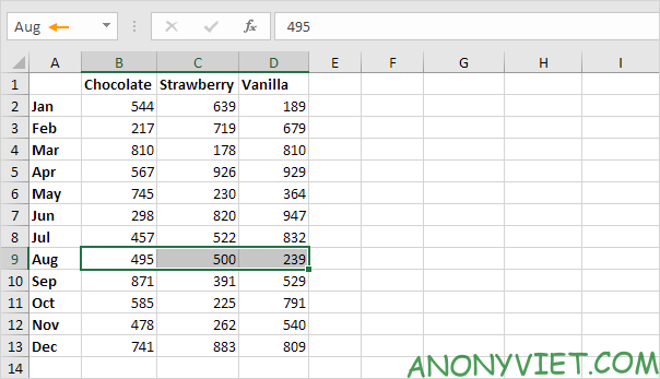
8. Excel created 12 + 3 = 15 range names! Just select a range and look at Name.
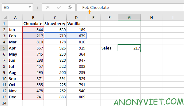
9. Use the intersection operator (space) to return the intersection of two zone names.
10. Create dynamic two-way lookups.
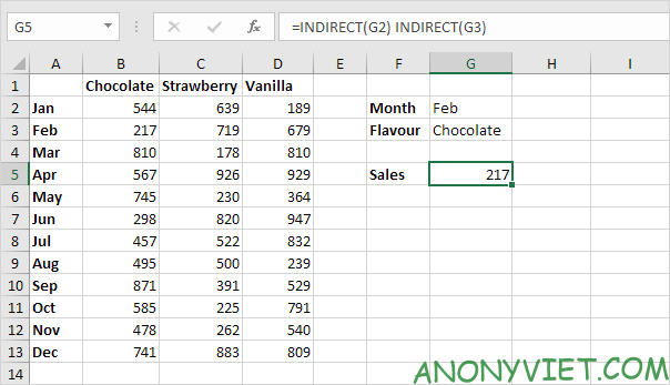
Explanation: the INDIRECT function converts text strings (“Feb” in cell G2 and “Chocolate” in cell G3) into valid named ranges.
In addition, you can also view many other excel articles here.


