In this article, I will show you how to use the . function SUMMARY in Excel to sum cells.
| Join the channel Telegram of the AnonyViet 👉 Link 👈 |
How to use the SUM function in Excel
Normally, you would use the SUM function in Excel to sum a range of cells.
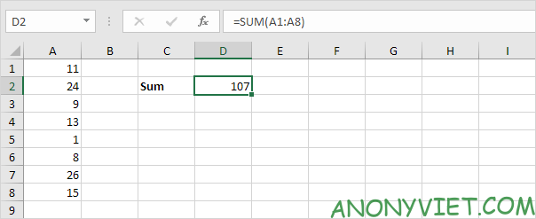
You can also use the SUM function in Excel to sum a column.
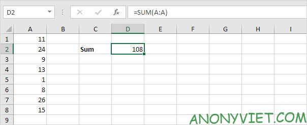

Note: you can also use the SUM function in Excel to sum entire rows. For example, =SUM(5:5) sums all values in the 5th row.
You can also use the SUM function in Excel to sum cells that are not contiguous, that is, not next to each other.
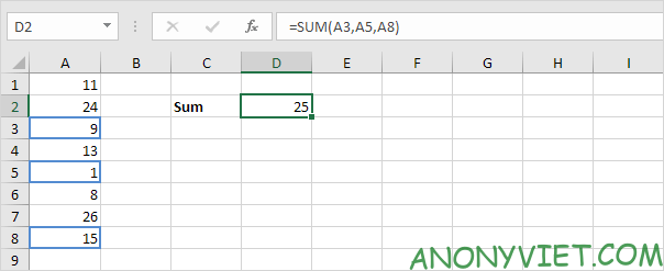
Note: =A3 + A5 + A8 gives the same result.
AutoSum
Use AutoSum or press ALT + = to quickly sum a column or row of numbers.
1. First, select the cell below the column of numbers (or next to the row of numbers) you want to sum.
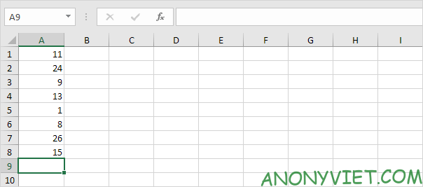
2. On the Home tab, in the Editing group, click AutoSum (or press ATL + =).

3. Press Enter.
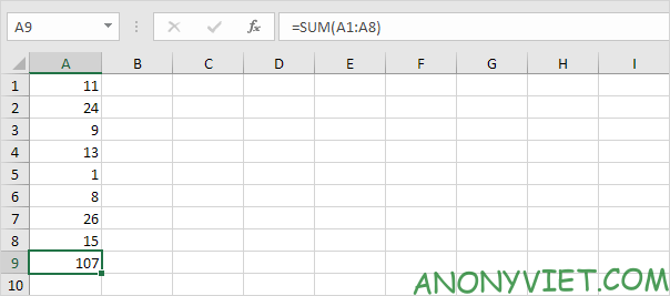
Calculating total goods
The SUM formula below uses SUM, MOD, and ROW to sum every nth row. Changing 3 to 4 will sum every 4th row, to 5 to sum every 5th row, etc.
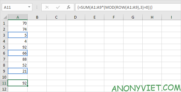
Note: this is an array formula enclosed in curly braces {}. Don’t type these yourself. To enter an array formula, finish by pressing CTRL + SHIFT + ENTER.
Add the largest numbers
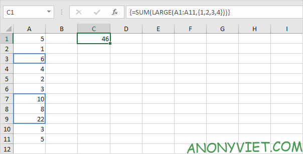
The SUM formula below uses SUM and LARGE to sum the largest numbers in a range. Change {1,2,3,4} to {1,2,3,4,5} to sum the largest 5 numbers.
Sum cells with no errors
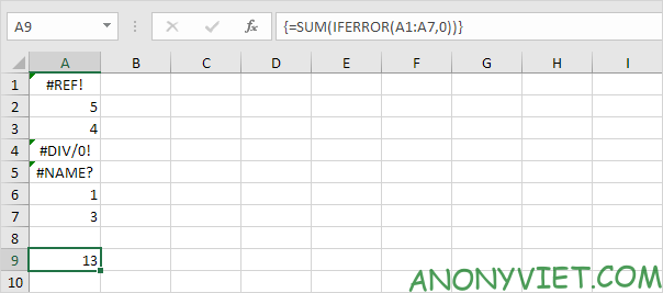
The SUM formula below uses SUM and IFERROR to sum a range of cells with errors. You can also use the Excel AGGREGATE function to sum an error range.
In addition, you can also view many other excel articles here.


