With conditional formatting in Microsoft Excelyou can highlight gaps or errors in Microsoft Excel to find them easier.
| Join the channel Telegram of the AnonyViet 👉 Link 👈 |

How to automatically highlight blank cells in Excel
When you have a spreadsheet full of data and want to fill every cell so you don’t have to deal with incorrect data. Here’s how to view blank cells using conditional formatting.
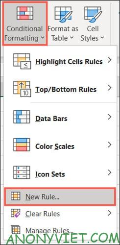
Open the worksheet and select the cells to which you want to apply the formatting. Go to the Home tab and click “Conditional Formatting” in the Styles group. Select “New Rule”.
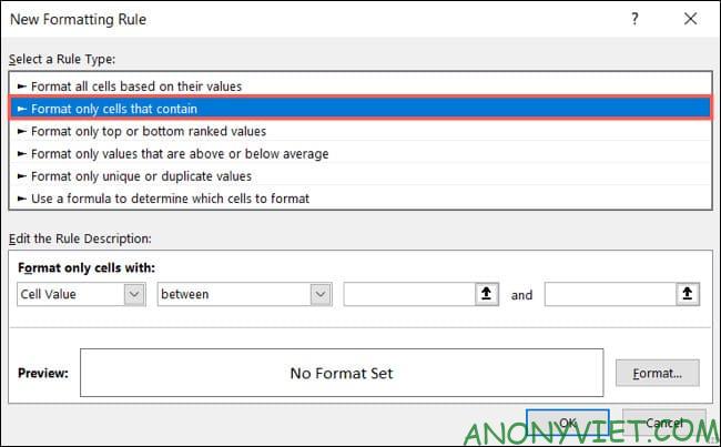
In the New Formatting Rule window, select “Format Only Cells That Contain” under Select a Rule Type.
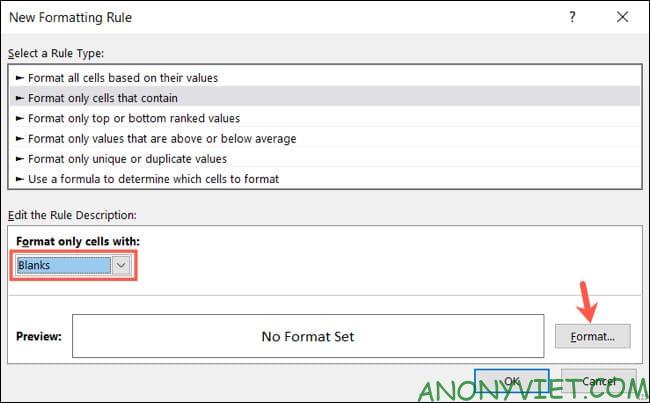
At the bottom, select “Blanks” under Format Only Cells. Then, click “Format” on the right to choose how to format the blank cells.
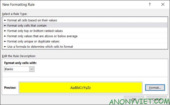
In the Format Cells window, you can use the Font, Border, and Fill tabs to choose the format you want. Click “OK”. I will use Fill to fill the empty cells with yellow.

Click “OK” to apply conditional formatting.
You will then see any empty cells in the range you selected highlighted in yellow.

How to automatically highlight errors in Excel
If you have a large, data-heavy sheet, you’ll need to flag errors to make them easier to spot.
Highlighting errors in Excel does the same thing as above, but a little differently.
Switch to the Home tab, click “Conditional Formatting”, then select “New Rule”.
In the New Formatting Rule window, select “Format Only Cells That Contain” at the top. But this time, select “Errors” under Format Only Cells With.
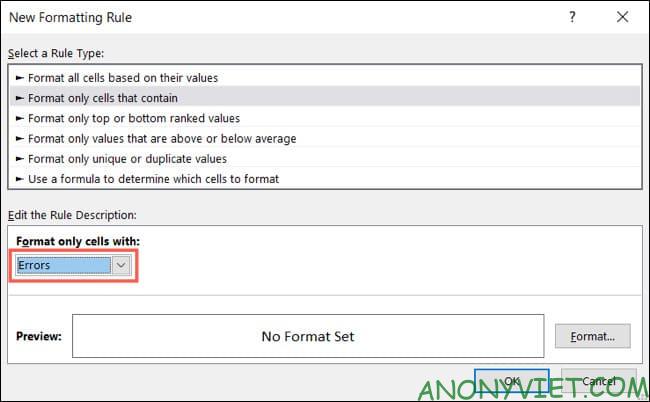
Then, click “Format” to choose a format. For this example, I will use the Font option to make the cells with errors bold and red. Click “OK” after you select the format and “OK” again to apply the format.
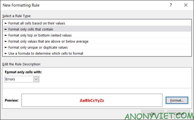
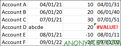
Now you can better identify the error.
You can also use this type of formatting in Microsoft Excel to do many other things. In addition, you can also Compare the content of 2 Excel files here.


