Lesson 33: How to use Freeze Panes – Fix columns when scrolling in Excel

If you have a large data table in Excel, it can be very helpful to freeze rows or columns. This way you can keep rows or columns visible while scrolling the sheet. So in this article, I will guide you to do the same using Freeze Panes.

How to use Freeze Panes in Excel

1. On the View tab, in the Windows group, and click Freeze Panes.

2. Click Freeze Top Row.

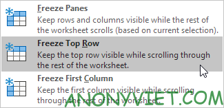
3. Scroll down the rest of the sheet.

Result: Excel automatically adds a dark gray horizontal line to indicate that the top row is fixed.

Unlock all rows and columns

To unlock all rows and columns, perform the following steps.

1. On the View tab, in the Windows group, select Freeze Panes.

2. Click Unfreeze Panes.

Fixed first column

To freeze the first column, perform the following steps.

1. On the View tab, in the Windows group, select Freeze Panes.

2. Click Freeze First Column.

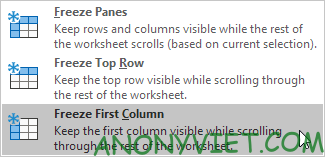
3. You can now scroll to the right of the sheet to see the difference.

Result: Excel automatically adds a dark gray vertical line to let you know that the first column is fixed.

Fixed row

To freeze the row, perform the following steps.

1. In this example, I will select row 4.

2. On the View tab, in the Windows group, select Freeze Panes.

3. Click Freeze Panes.

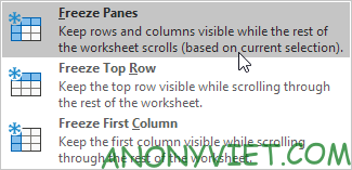
4. Scroll the sheet and see the results.

Result. All rows above row 4 are fixed. Excel automatically adds a dark gray horizontal line to let you know that the first three rows are fixed.

Fixed column

To freeze columns, perform the following steps.

1. In this example, I will select column E.

2. On the View tab, in the Windows group, select Freeze Panes.

3. Click Freeze Panes.

4. Scroll the sheet and see the results.

Result: All columns to the left of column E are fixed. Excel automatically adds a dark gray vertical line to indicate that the first four columns are fixed.

Fixed umbrella

To freeze the cell, perform the following steps.

1. In this example, I will select cell C3.

2. On the View tab, in the Windows group, select Freeze Panes.

3. Click Freeze Panes.

4. Scroll the sheet and see the results.

Result: The orange area above row 3 and to the left of column C was frozen.

How to Add Freeze Panes Shortcut to Quick Access

Add a magic Fix button to the Quick Access Toolbar to freeze the top row, first column, rows, columns, or cells with a single click.

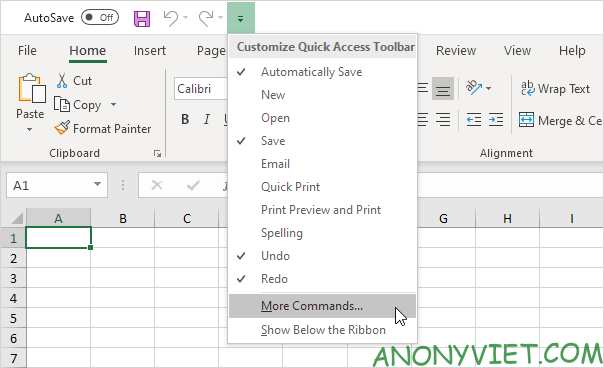
1. Tap the down arrow.

2. Select More Commands.

3. In Choose commands from, select Commands Not in the Ribbon.

4. Select Freeze Panes and click Add.

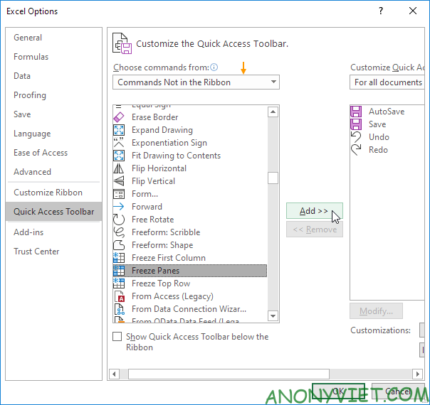
5. Press OK

6. To freeze the top row, select row 2 and click the Freeze button.

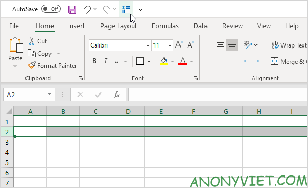
7. Scroll the sheet and see the results.

Result: Excel automatically adds a dark gray horizontal line to let you know that the top row is fixed.

Note: to unlock all rows and columns, click the Freeze button again. To freeze the first 4 columns, select column E (the fifth column) and click the Freeze button.

In addition, you can also view many other excel articles here.