This article will show you how to apply strikethrough formatting in Excel. You can still read the text with the strikethrough effect.
| Join the channel Telegram of the AnonyViet 👉 Link 👈 |
How to strikethrough in Excel
1. For example, select range A2:A4.
2. Right-click, and then click Format Cells (or press Ctrl + 1).
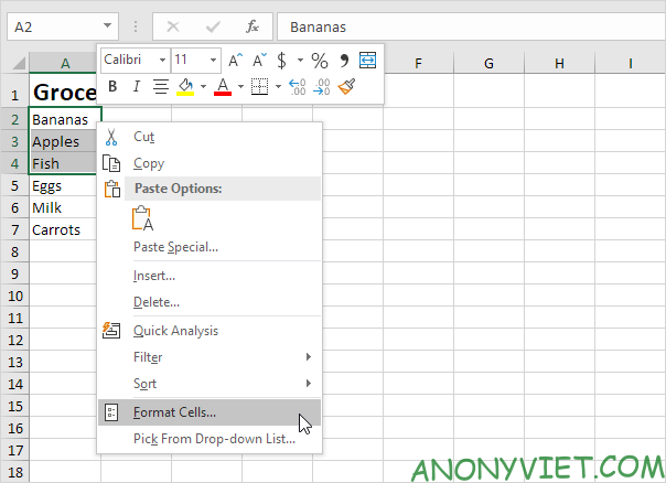
3. On the Font tab, under Effects, click Strikethrough.
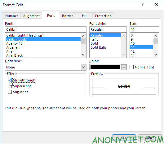
4. Click OK.
Result:
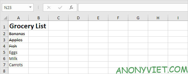
You can also use keyboard shortcuts to quickly apply strikethrough formatting in Excel.
5. For example, select cell A7.
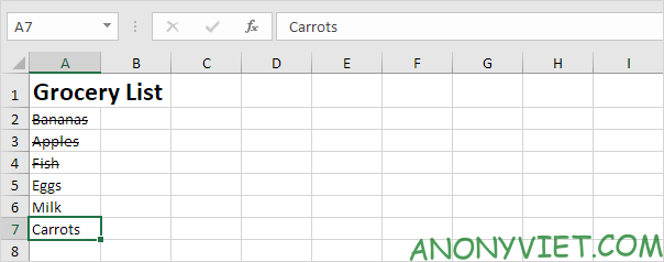
6. Press Ctrl + 5.
Result:
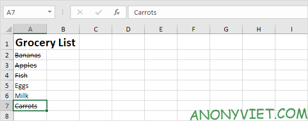
Note: just press Ctrl + 5 again to remove the strikethrough effect. There is no double strikethrough option in Excel.
7. To apply strikethrough formatting to only part of a cell, first select that text in the formula bar.

8. Press Ctrl + 5.

Let’s see 2 more apply quick strikethrough formatting in Excel.
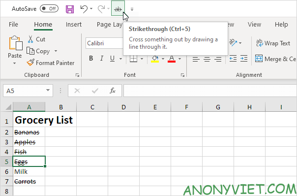
9. Add a strikethrough button to the Quick Access Toolbar.
10. Select cell A5 and click the strikethrough button.
11. Add the following lines of code BeforeDoubleClick Event:
Target.Font.Strikethrough = True
Cancel = True
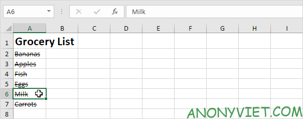
12. Double-click cell A6.
In addition, you can also view many other excel articles here.


