This article will show you how to create a measurement chart in Excel.
| Join the channel Telegram of the AnonyViet 👉 Link 👈 |
Measurement chart in Excel
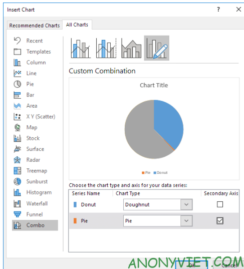
To create a measurement chart, do the following:
1. Select range H2: I6
2. On the Insert tab, click the Combo icon.

3. Click Create Custom Combo Chart.

4. For the Donut series, select Donut as the chart type.
5. For Pie series, select Pie as the chart type.
6. Draw the Pie chain on the second axis.

7. Press OK
8. Remove chart title and legend.
9. Select the chart. On the Format tab, select Pie Series.

10. On the Format tab, click Format Selection and change the angle of the first slice to 270 degrees.
11. Hold down CTRL and use the ← and → keys to select a data point. On the Format tab, change the Shape Fill of each point. Score 1 = No fill, point 2 = black and point 3 = No fill.
Result

12. Repeat steps 9 to 11 for the Donut series. Score 1 = red, point 2 = yellow, point 3 = green and point 4 = No fill.
Result

In addition, you can also view many other excel articles here.


