Using the IFERROR function in Excel to return an alternate result, such as text, when the formula fails.
| Join the channel Telegram of the AnonyViet 👉 Link 👈 |
How to use the IfError function in Excel
1. For example, Excel returns #DIV/0! error when a formula tries to divide a number by 0.

2. If the formula fails, the IFERROR function below returns what you want.

3. If the formula has no errors, the IFERROR function only returns the result of the formula.

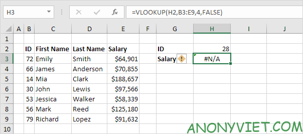
4. For example, Excel returns the #N/A error when the VLOOKUP function cannot find a match.

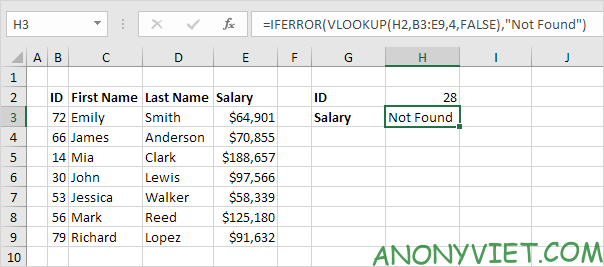
5. If the Vlookup function returns an error, the IFERROR function below returns what you want.

6. If the VLOOKUP function fails, the IFERROR function only returns the result of the VLOOKUP function.

Note: the IFERROR function catches the following errors: #DIV/0!, #N/A, #VALUE!, #REF!, #NUM!, #NAME? and #NULL!. For example, the IFERROR function shown above also catches the #NAME? if you accidentally misspelled the word VLOOKUP. Use the IFNA function in Excel 2013 and later to catch only #N/A errors.
In addition, you can also view many other excel articles here.


