Lesson 154: How to use the Vlookup function in Excel

The Vlookup function is one of the most popular lookup functions in Excel.

How to use the Vlookup function in Excel

Precise detection

1. The VLOOKUP function below looks up the value 53 (first parameter) in the leftmost column of the red table (second parameter).

2. The number 4 (third parameter) tells the VLOOKUP function to return the value of the fourth column in the red table.

Note: Boolean FALSE (fourth parameter) requires the VLOOKUP function to return an exact result. If the VLOOKUP function cannot find the value 53 in the first column, it returns the #N/A error.

3. Here is another example. Instead of returning the salary, the VLOOKUP function below returns the last name (the third parameter is set to 3) of ID 79.

Approximate detection

1. The VLOOKUP function below looks up the value 85 (first parameter) in the leftmost column of the red table (second parameter). But the problem is that there is no value 85 in the first column.

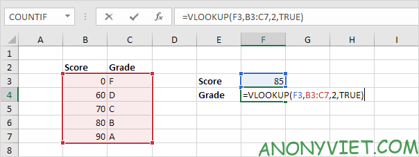
2. Fortunately, TRUE (the fourth parameter) tells the VLOOKUP function to return an approximate match. If the VLOOKUP function cannot find the value 85 in the first column, it will return a value less than 85. In this example, this would be the value 80.

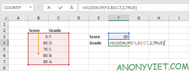
3. Number 2 (third argument) tells the VLOOKUP function to return the value of the second column in the red table.

Note: always sort the first column of the red table in ascending order if you use the Vlookup function in approximate detection mode (the fourth parameter is set to TRUE).

How it works

The VLOOKUP function always looks up the value in the leftmost column of the table and returns the corresponding value from the right column.

1. For example, the VLOOKUP function below looks up the first name and returns the last name.

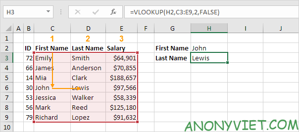
2. If you change the 3rd parameter to 3, the VLOOKUP function will look up the name and return the salary.

Note: in this example, the VLOOKUP function cannot look up the name and return the ID. The Vlookup function only looks from left to right. Don’t worry, you can use INDEX and MATCH in Excel to do a left lookup.

Duplicate value

If the leftmost column of the table has the same value, the VLOOKUP function returns the first result. For example, the Vlookup function below.

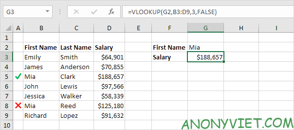
Explanation: the VLOOKUP function returns Mia Clark’s salary, not Mia Reed’s.

Vlookup is not case sensitive

The VLOOKUP function in Excel performs case-insensitive detection. For example, the VLOOKUP function below looks up the MIA (cell G2) in the leftmost column of the table.

Explanation: the VLOOKUP function is not case sensitive so it will look up MIA or Mia or mia or miA… As a result, the VLOOKUP function returns Mia Clark’s salary (first case). Use INDEX, MATCH, and EXACT in Excel to perform case-sensitive lookups.

Many conditions

You can search based on multiple conditions by using INDEX and MATCH in Excel to perform a two-column lookup.

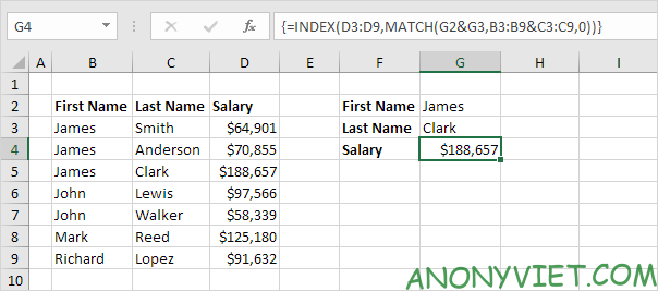
Note: the array formula above looks up James Clark’s salary, not James Smith’s, not James Anderson’s.

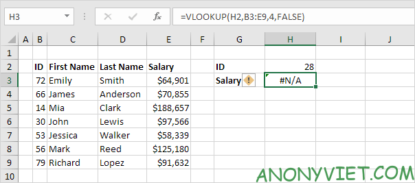
Error #N/A

If the VLOOKUP function cannot find a match, it returns the #N/A error.

1. For example, the VLOOKUP function below cannot find the value 28 in the ID column.

2. If you want, you can use the IFNA function to replace the #N/A error with what you want.

Note: the IFNA function was introduced in Excel 2013. If you are using Excel 2010 or Excel 2007, just replace IFNA with IFERROR.

Look up multiple tables

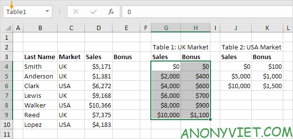
When using the Vlookup function in Excel, you can look up more tables. You can use the IF function to check if a condition is met and return a lookup table if TRUE and another lookup table if FALSE.

1. Create two range names: Table1 and Table2.

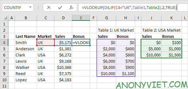
Explanation: Bonus depends on Market (UK or US) and sales quantity. The second parameter of the VLOOKUP function determines the lookup table. If UK, the VLOOKUP function uses Table1, if USA, the VLOOKUP function uses Table2. Set the fourth parameter of the VLOOKUP function to TRUE to return an approximate result.

3. Press Enter.

4. Select cell E4, click the lower right corner of cell E4 and drag it down to cell E10.

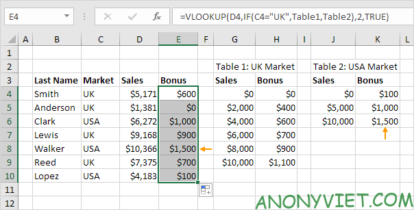
Note: for example, Walker received a bonus of $1,500. Because I use the reference as the range name, there is no need to worry when copying the formula to another cell.

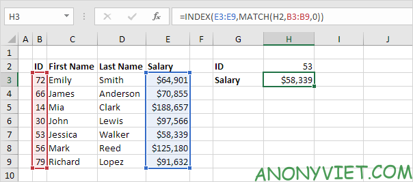
Index and Match

Instead of using the VLOOKUP function, use INDEX and MATCH. To perform advanced lookups, you will need INDEX and MATCH.

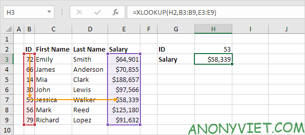
Xlookup

If you use Excel 365, use XLOOKUP instead of VLOOKUP. The XLOOKUP function is easier to use and has several additional advantages.

In addition, you can also view many other excel articles here.