Instructions to automatically color Excel cells according to conditions

Color scales represent all sorts of things like temperature, speed, age, and even population. If you want to apply this auto-coloring to Excel cells with the available condition, use the Color Scale feature according to the instructions below.

With conditional formatting, you can apply a gradient color scale in just a few minutes. Excel provides a two- and three-color color scale that you can choose from, along with other options for customizing your color scale.

Automatically color Excel cells with conditional formatting

Microsoft Excel provides you with several color scale templates to automatically colorize Excel cells for quick application. These include six two-color scales and six three-color scales.

Select the cells that you want to apply. Then go to section Styles of the Home tab.

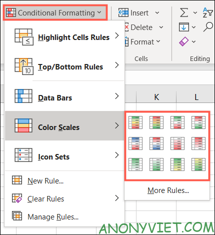
Click on “Conditional Formatting” and select “Color Scales.“. You will see all 12 color scale options available.

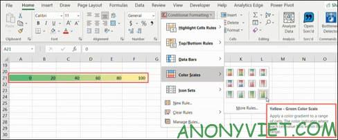
As you hover over each one, you’ll see the cells you selected change as well. Thanks to that, you can easily choose the most suitable color scale for your Excel table.

Customize conditional formatting color scale

If you don’t like Excel’s built-in color scale templates, you can still easily create your own color scale.

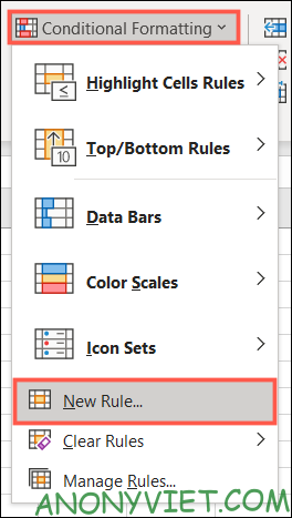
Select the cells you want, go to the Home tab and select “New Rule” under “Conditional Formatting”.

When the new New Formatting Rule window opens, select “Format All Cells Based on Their Values” at top.

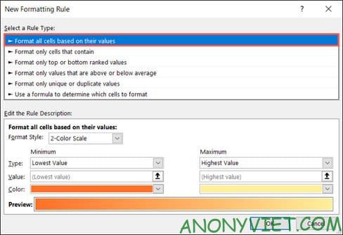
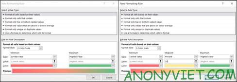
Part Edit the Rule Description At the bottom of the window is where you’ll spend time customizing the color scale rule. Start by choosing 2-Color Scale or 3-Color Scale (2 or 3 color scale).

The main difference between the two is that the tricolor scale has a midpoint, while the two color scale has only minimum and maximum values.

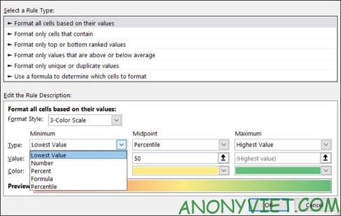
After choosing the color scale style, select Minimum, Maximum and Midpoint under Types. You can also choose from Lowest/Highest Value, Number, Percent, Formula, or Percentile.

The Lowest Value and Highest Value types are based on the data in the selected cell range, so you don’t need to enter anything. Excel will automatically color the cells according to the condition.

Finally, click Color to choose the color you want. If you want to customize the colors, select “More Colors” to use RGB or Hex color codes.

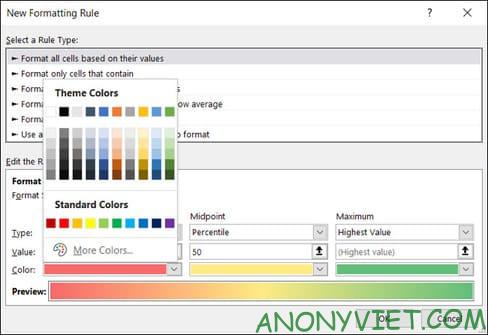
You will then see a preview of your color scale at the bottom of the window. If you are satisfied with the results, press “OK” to apply the formatting.

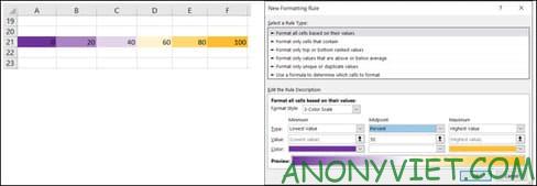
If you edit your data, the color scale will automatically update to accommodate the change.

So you have successfully applied the color scale in Microsoft Excel. In addition, you can also learn Excel quickly with these 8 tips.