To find the best match to the target value in a data column, use INDEX, MATCH, ABS, and MIN in Excel. Using the Vlookup function in Excel to find approximate results.
| Join the channel Telegram of the AnonyViet 👉 Link 👈 |
Find the best match in Excel
1. The ABS function in Excel returns the absolute value of a number.
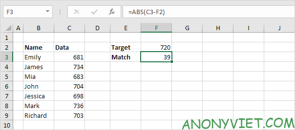
2. To calculate the difference between the target value and the values in the data column, replace C3 with C3:C9.
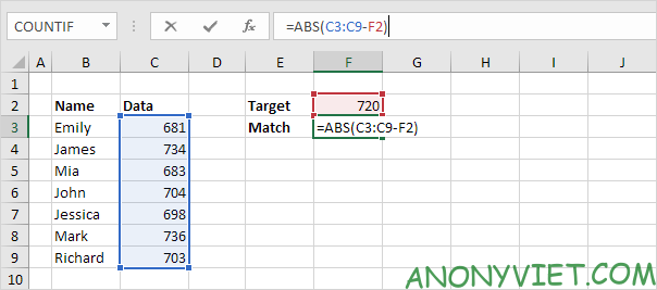
Explanation: the range (array constant) generated by the ABS function is stored in Excel’s memory, not in the range. The array constant looks like this:
{39;14;37;16;22;16;17}
3. To find the best match, add the MIN function and finish by pressing CTRL + SHIFT + ENTER.
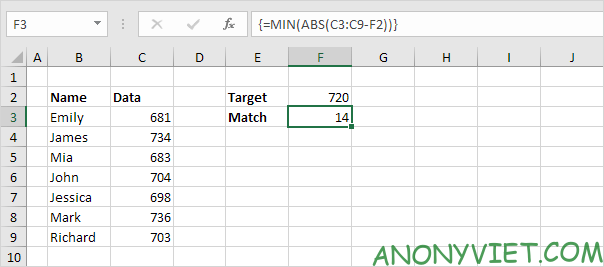
4. All we need is a function that finds the position of the value 14 in the array constant. You can use the MATCH function to do this.
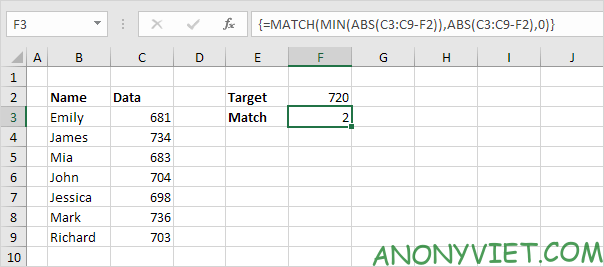
Explanation: 14 (first parameter) is found at position 2 in the array constant (second parameter). In this example, we use the MATCH function to return an exact match, so we set the third parameter to 0.
5. Use the INDEX function (two parameters) to return a specific value in a one-dimensional range. In this example, name is in position 2 (second argument) in the range B3:B9 (first argument).

6. Finish by pressing CTRL + SHIFT + ENTER.

In addition, you can also view many other excel articles here.

