By default, the VLOOKUP lookup function is case-insensitive. However, you can use INDEX, MATCH and EXACT in Excel to do a case-sensitive lookup.
| Join the channel Telegram of the AnonyViet 👉 Link 👈 |
Case sensitive lookup in Excel
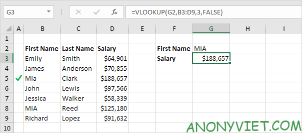
1. For example, the simple VLOOKUP function below returns Mia Clark’s salary. However, I want to look up the salary of MIA Reed (see cell G2).
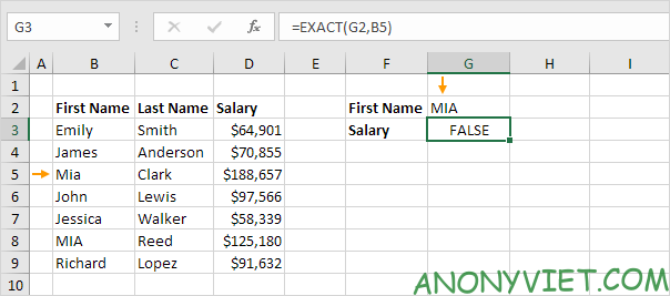
2. The Excel EXACT function returns TRUE if the two strings are exactly the same. So the EXACT function below will return FALSE.
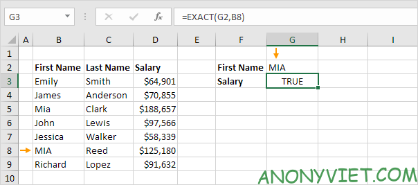
3. The EXACT function below returns TRUE.
4. Replace B8 with B3:B9.
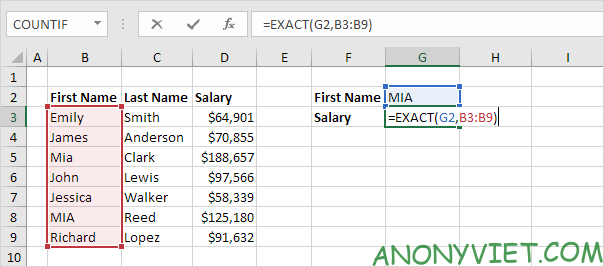
Explanation: The range (array constant) created by the EXACT function is stored in Excel’s memory, not in a range. The array constant looks like this:
{FALSE;FALSE;FALSE;FALSE;FALSE;TRUE;FALSE}
5. All we need is a function that finds the position of TRUE in this array constant. And the MATCH function can do this.
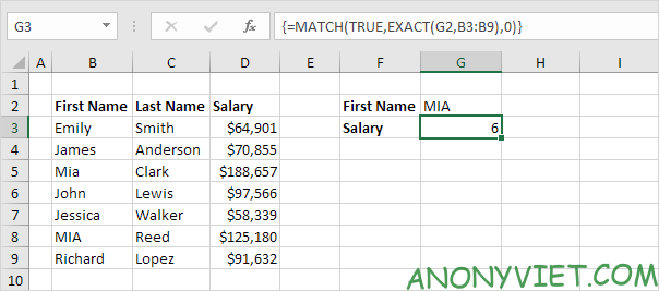
Explanation: TRUE (first parameter) is found at position 6 in the array constant (second parameter). In this example, we use the MATCH function to return the correct result, so we set the third parameter to 0. The formula bar indicates this is an array formula by enclosing it in curly braces. {}.
6. Use the INDEX function to return a specific value in a one-dimensional range. In this example, the salary is at position 6 (second parameter) in the range D3:D9 (first parameter).
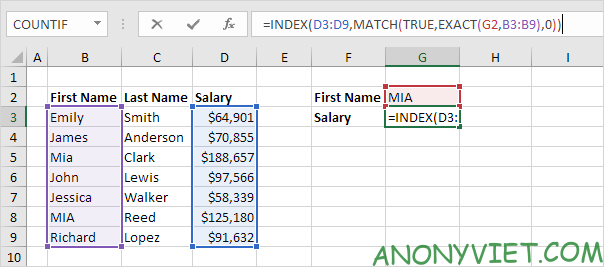
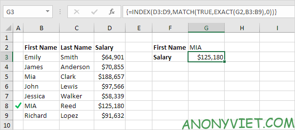
7. Finish by pressing CTRL + SHIFT + ENTER.
In addition, you can also view many other excel articles here.

