Sorting and filtering data will help you get rid of unnecessary data and find (or sort) the data you want to see. Microsoft Excel will make you happy with the huge data filter options and simple sorting ways.

How to sort data in Excel
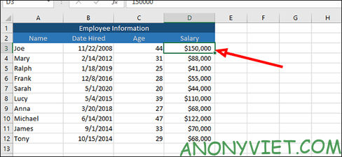
The first step to sorting and filtering that data is to determine how you want to sort. You can see a specific example like this: We will click on cell D3 and sort this column by salary.
Then select “Data” and click “Filter”.
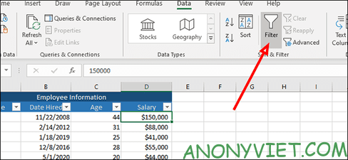
Now on each column you will see an arrow appear. Click the arrow of the column you want to sort to display a sorted or filtered list of data.
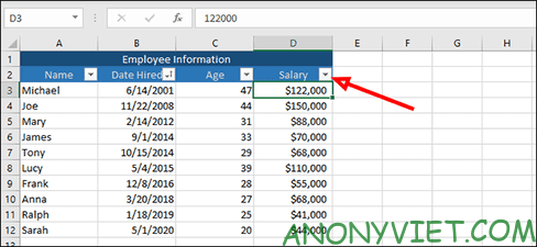
The simplest data sort is from smallest to largest or largest to smallest. In the example you saw above, we are sorting salary, so we will sort from smallest to largest. best.
We can also apply the same sort to any other column.
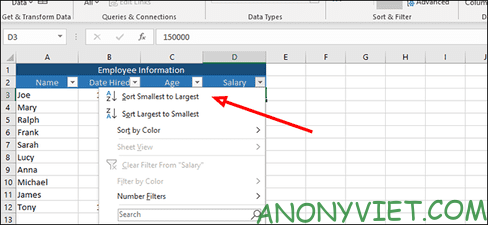
For example, sort by rental date by selecting “Sort Oldest to Newest”.
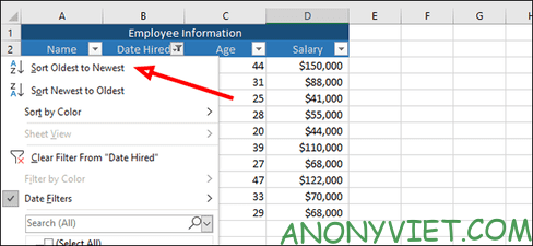
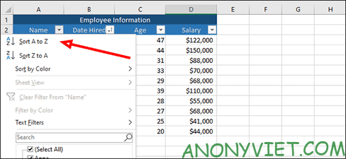
These data sorting options also work for the “Age” and “Name” columns. For example, we can sort by age from oldest to youngest, or sort employee names alphabetically by clicking on the arrow and selecting the appropriate option.
How to filter data in Excel
The steps above are just sorting to prepare for the next data filtering operation. Now we will learn how to filter data very easily with just a few quick steps.
First, click the arrow next to “Salary” to filter this column. In this example, we’ll filter out anyone making more than $100,000 per year.

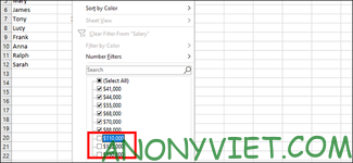
Since our list is short, we can make this step very simple. The first way, which works very well in the example above, you simply uncheck each person who earns more than $100,000 and then press “OK”. This will remove three items from the list and allow us to view (and sort) the remaining items.
The second way is simpler, press the arrow key next to “Salary” again.
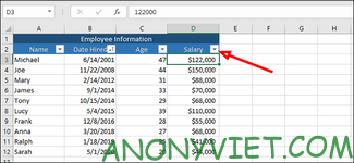
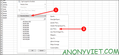
This time, we will click on “Number Filters” and choose “Less Than”.
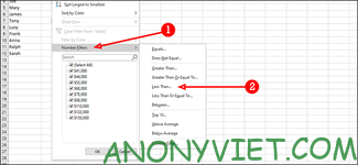
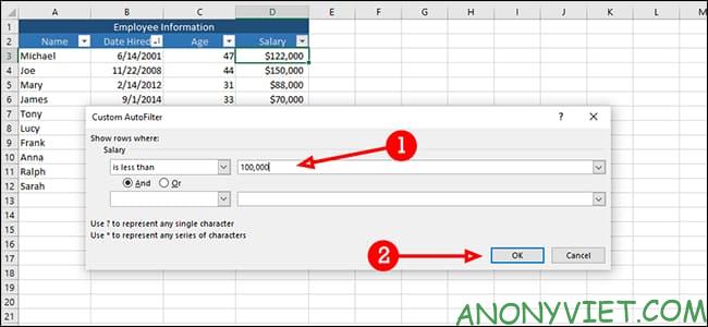
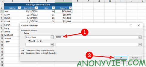
Here we can also filter the results like excluding anyone who earns more than $100,000 per year. But this works much better for large data sets, you don’t need to do a lot of manual clicking to remove items. To the right of “is less than”, enter “100,000” (or whatever number you want) and then press “OK”.
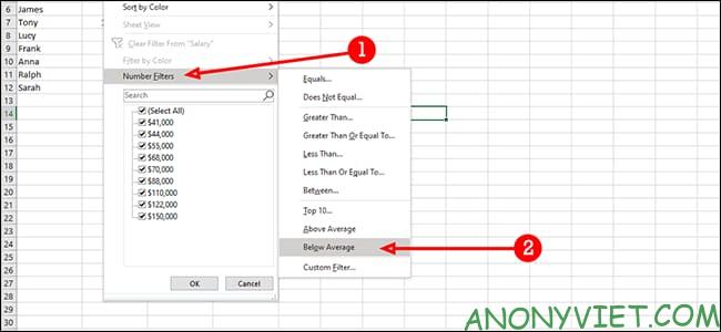
We can also use this filter for other purposes. For example, we can filter out all salaries above average by clicking “Below Average” from the list (Number Filters > Below Average).
We can also combine filters together. Here, we’ll find all salaries greater than $60,000 but less than $120,000. First, select “is greater than”.
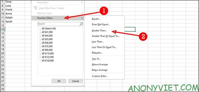
Next select “is less than.”
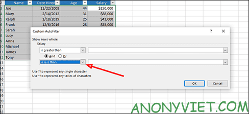
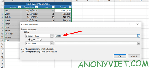
In the “is greater than” field, enter 60,000.
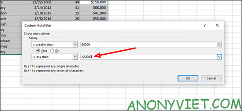
Next in the “is less than” field enter 120,000.
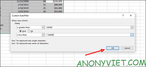
The final step is to hit “Ok” to filter your data, and once done, you will see salaries greater than $60,000 and less than $120,000.
How to filter data from multiple columns at once in Excel
In this example, we will filter by date of hire and salary. We’re looking for people who were hired after 2013 and make less than $70,000 per year.
The first step is to click the arrow next to the “Salary” box to filter out anyone making $70,000 or more per year.

Next click on “Number Filters” and finally select “Less Than.”
Enter 70,000 next to “less than” and select “Ok” to finish.
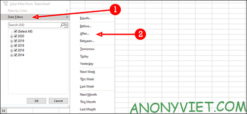
Next, we’ll filter by the date each employee was hired, excluding those hired after 2013. Click the arrow next to “Date Hired”, then select “Date Filters” and then select “After”.
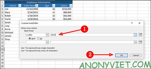
Type “2013” to the right of “is after” then press “OK”. This step will filter out employees who earn less than $70,000 per year and were hired in 2014 or later.
Excel has a number of very efficient sorting and filtering options, and each is as customizable as you need it to be. Alternatively, you can also learn the free Excel course here.


