Microsoft Excel is a commonly used, full-featured spreadsheet application, but it’s far from perfect. Excel’s longtime rival is Google Sheets provides features that Excel does not, including a lot of useful functions. ![]()
This list is not all-inclusive, and Excel may add one or more of these functions at any time. But as of this writing in May 2022, here are the Google Sheets functions I’d like to see in Microsoft Excel. I will also show you how to use each function in Google Sheets.
Basic Calculations: ADD, MINUS, MULTIPLY, and DIVIDE
You can certainly add, subtract, multiply, and divide numbers in Microsoft Excel. However, these common operations are performed using formulas and operators, not functions. Excel provides a SUM function, which works like ADD, but Google Sheets has a clear and unified collection of functions to make it easier to work with.
The syntax for each function in Google Sheets is the same with the function name and two arguments: ADD(value1, value2), MINUS(value1, value2,). You can insert values, use cell references, or enter a combination of the two.
To subtract the values in cells A1 and A2, you can use the following formula:
=MINUS(A1,A2)
To subtract cell A1 by 10, you can use the following formula:
=MINUS(A1,10)
To calculate 20 minus 10, you can use the following formula:
=MINUS(20,10)

Count unique values: COUNTUNIQUE
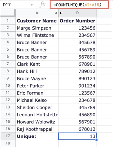
If you need to count the number of distinct values in Google Sheets, then COUNTUNIQUE is the function for you. Count how many customers ordered once, products with no inventory, or anything else you want to have unique value using this function.
The syntax of the function is COUNTUNIQUE(value1, value2, …) where the first argument is required. You can use cell references or values.
To find the number of unique customers in the range A1 to A16. We can see the number of people who ordered one time using the function:
=COUNTUNIQUE(A1:A10)

To count unique values in a list of inserted values, you can use this formula:
=COUNTUNIQUE(1,2,3,3,3,4)

Language Functions: DETECTLANGUAGE and GOOGLETRANSLATE
Google Sheets is more than just numbers and calculations. You may be working on a worksheet with people who speak another language. With DETECTLANGUAGE you can define the language of the text and with GOOGLETRANSLATE you can translate the text into another language.
The syntax for the first function is DETECTLANGUAGE(text) where you can enter actual text or cell references.
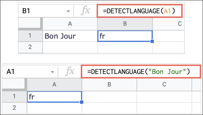
To determine the language in cell A1, you can use the following formula:
=DETECTLANGUAGE(A1)
To determine the language of specific text, you would use this function with your own text inserted between quotes:
=DETECTLANGUAGE("Bon Jour")

The syntax for the second function is GOOGLETRANSLATE(text, from_language, to_language), you can use cell reference or text for the first parameter. For language parameters, you need to use two-letter abbreviations. You can also use “auto” for the from_language argument to automatically detect the source language.
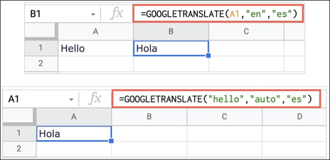
To translate the text in cell A1 from English to Spanish, use the following formula:
=GOOGLETRANSLATE(A1,"en","es")
To translate a certain phrase into Spanish using automatic language detection, you can use the following formula:
=GOOGLETRANSLATE("Hello","auto","es")

Greater than, less than and equal to: GT, GTE, LT, LTE, EQ
Excel does this too, but it’s more complicated. In Google Sheets, you can simply use the functions:
- GT: Greater than, syntax
GT(value1, value2) - GTE: Greater than or equal to, syntax
GTE(value1, value2) - LT: Less than, syntax
LT(value1, value2) - LTE: Less than or equal to, syntax
LTE(value1, value2) - EQ: Equals, syntax
EQ(value1, value2)
The formula for each function returns True or False. For example, if value1 is greater than value2, you will get True. Otherwise you will get False.
To see if the value in cell A1 is greater than the value in cell A2, you can use the following formula:
=GT(A1,A2)
To see if the first value is greater than the second, you can use the following formula:
=GT(4,5)
To see if the value in cell A1 is greater than the value provided, you can use the following formula:
=GT(A1,5)

Insert and customize images: IMAGE
Along with numbers and text, you can also insert pictures into your spreadsheet. While you can easily insert a picture into Google Sheets, the IMAGE function allows you to insert a picture from the web and then customize the size of that image.
The syntax of the function is IMAGE(url, mode, height, width) where only the first parameter is required. Here are the options you can use for the mode parameter:
- 1: Adjust the image in the cell and maintain the aspect ratio. This is the default mode.
- 2: Stretch or squeeze the image to fit the cell without maintaining the aspect ratio.
- 3: Keep the image in its original size.
- 4: Use a custom size by entering the height and width arguments in pixels.
To insert from the web and keep the original size, you can use this formula and replace the URL with your own:
=IMAGE("https://www.howtogeek.com/wp-content/uploads/2022/02/DateOptions-GoogleSheetsCustomDateTime.png",3)

To insert the same image but using a custom size, you can use this formula and change the URL, width and height to your liking:
=IMAGE("https://www.howtogeek.com/wp-content/uploads/2022/02/DateOptions-GoogleSheetsCustomDateTime.png",4,200,500)

Add a little graph: SPARKLINE
You don’t always need a large graph in your spreadsheet. Google Sheets allows you to add a mini chart using the SPARKLINE function. In Excel, you can create curves using the chart feature, but this function is simpler and faster.
The syntax is SPARKLINE(data, custom) where only the first parameter is required.
To add a basic bend with data from cell range B2 to E2, you can use the following formula:
=SPARKLINE(B2:E2)

To use a column chart with the same range of cells, you can use the following formula:
=SPARKLINE(B2:E2,{"charttype","column"})

In addition, you can also see more about many other functions in google sheets here.


